Contents
|
|
new 1D techniques: CSSF 1D-TOCSY and CSSF 1D-NOESY |
|
|
Department of Chemistry,
University of Alberta March
2008
NMR News 2008-01
News and tips from the NMR support group for users of the Varian NMR systems in the
Department
Editor: Albin.Otter@ualberta.ca
http://nmr.chem.ualberta.ca
There are no fixed publishing dates for this newsletter; its appearance solely depends on whether there is a need to present information to the users of the spectrometers or not.
Other content of this NMR News is no longer meaningful and has been removed May 2010.
|
Contents
|
new 1D techniques: CSSF 1D-TOCSY and CSSF
1D-NOESY
1D versions of 2D techniques have the advantage of providing the desired
spectral information with higher spectral quality due to higher
digital resolution and
higher signal-to-noise ratios (the latter is only relevant when working with
dilute samples). They require waveform generator hardware and consequently the
i300 and m400
are not capable to do these techniques. All the others have the necessary
hardware, and the two techniques have been implemented already on the i600 and
ibd5 spectrometers with u500, i400 and s400 to follow soon.
 |
The disaccharide β-maltoside
α-Glc(1-4)β-Glc-OCH3 (shown on the left) is used throughout these notes for illustration purposes.
αH1
is at 5.4 ppm, |
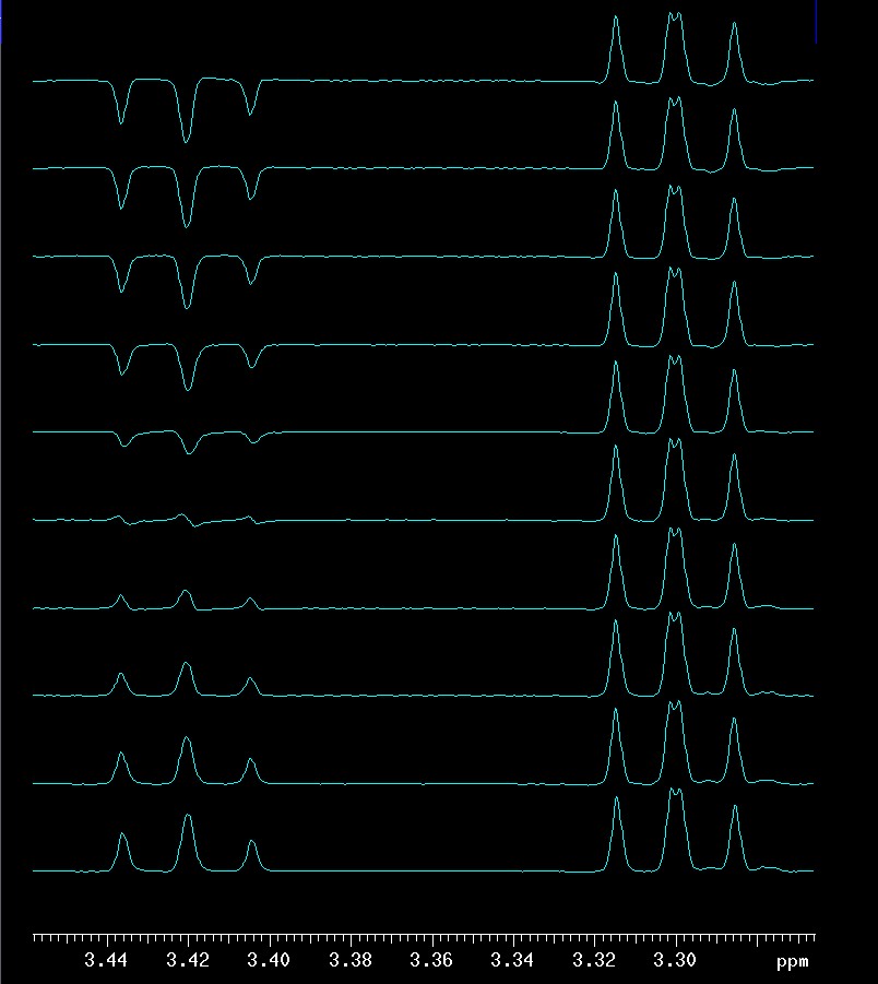
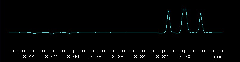
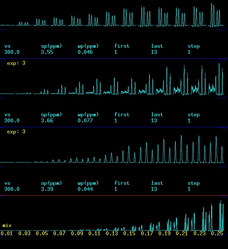
Both techniques use chemical shift selective filters (CSSF) to achieve very high selectivity. In a nutshell, CSSF techniques are pseudo-2D experiments. If the shift difference between a proton signal that should be selectively excited and one that has to be avoided is quite large, then it is simply a 1D with ni=1. With decreasing difference between desired and undesired signals, ni increases and accordingly the experimental time increases proportionally and selectivity is achieved through the addition of 1Ds (ni of them!). In the example below, the difference between the desired and undesired signal was only 6.4 Hz and ni ended up as 10 (the program calculates ni automatically, based on user input shown later). The 10 traces are shown here only for illustrative purposes. Normally there is little interest in seeing these traces. What is evident is how the signal that is part of the selected spin system at 3.30 ppm (it is βH2) is always positive while the other one at 3.42 ppm (αH4) is much weaker and inconsistent in phase (some up, some down, some almost zero). After using the command proc_cssf (or using the WFT button in EZ NMR which will execute proc_cssf automatically in CSSF techniques), the traces are co-added and the spectrum shown as a separate picture at the bottom is the net result: the undesired signal cancels out almost completely while the desired one is more intense relative to the spectral noise which is hard to see here because the s/n is high.
 |
 |
|
top: 10 traces of the ni=10
CSSF 1D-TOCSY with selective excitation of
βH3
at 3.78 ppm and a mixing time of 0.120 seconds |
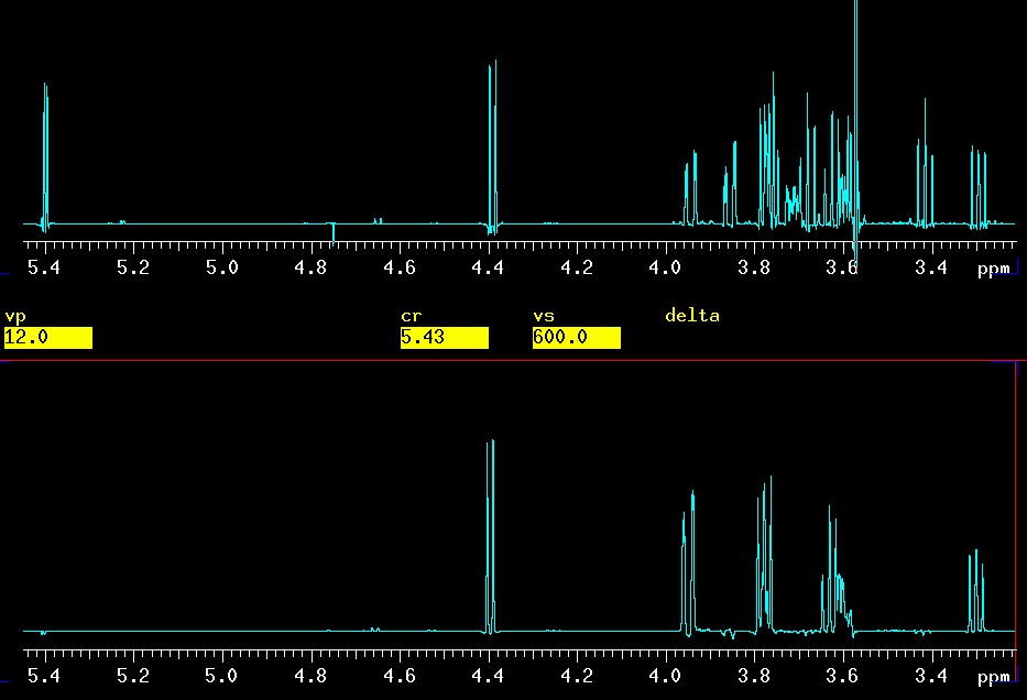
This is quite an extreme example with only 6.4 Hz separation but not a record. Signals as close as 2 Hz have been selectively excited but with overnight experimental times. With ni=10 and nt=32, this experiment took a little longer than 30 minutes which is is not much time considering that the two spin systems were completely separated as shown below (1D on top, entire β-Glc sub-spectrum below):
 |
|
top: 1D spectrum |
Again, just to demonstrate the feasibility, the selective excitation started in the worst possible place of the spectrum with the most overlap around 3.78 ppm. The H3 of the β-Glc ring at 3.78 ppm was selectively excited and all protons of the β-Glc ring appeared cleanly [in ppm]: H1 4.4, H2 3.3, H3 3.78, H4 3.63, H5 3.60 and the two H6a/b at 3.95 and 3.78 (H3 and H6b are virtually identical in chemical shift).
The easy way would have been to hit either βH1 at 4.4 or βH2 at 3.2 and the experiment could have been done with ni=1 nt=32 in roughly 3 minutes. The result of precisely this experiment compared to the 1D on top is shown here:
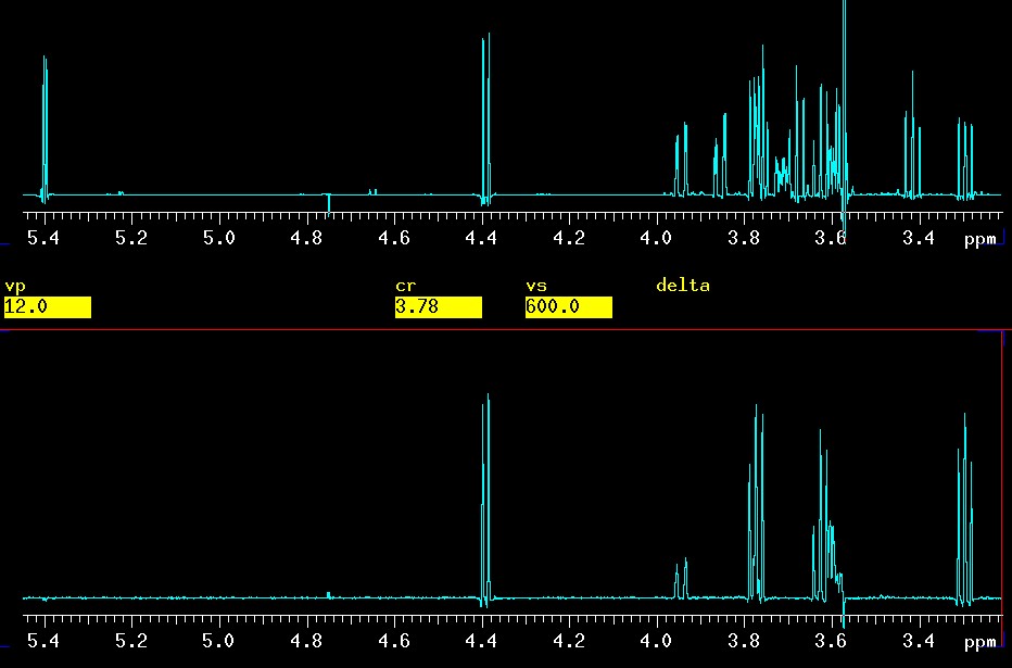 |
|
top: 1D spectrum |
The βH6a proton at 3.9 ppm is clearly visible with the mixing time of 0.120 seconds which is the same as used in the spectrum discussed earlier where βH3 was selectively excited. It is not surprising that βH6a is weaker when starting at βH1: there are five "steps" from H1 to H6, namely H1>-H2->H3->H4->H5->H6, but only three H3->H4->H5->H6 when H3 is selectively excited.
The far superior quality of the CSSF 1D-TOCSY can best be seen in a comparison with its 2D-GCOSY equivalent, shown below. The trace is taken through βH1 at 4.4 and in essence shows the same correlations as the 1D version. But, for example, βH2 at 3.3 ppm is a clean peak in the 1D-TOCSY and rather a mess in the 2D. Around 3.6 ppm the 2D decays completely due to overlap and lack of digital resolution while the 1D equivalent is very clean.
The real "selling point" (no worries, you can use it for free!) of this technique is the fact that coupling constants can be extracted with high precision, typically +/- 0.1 Hz. This is not possible in the 2D versions of TOCSY (GTOCSY and others) because the digital resolution does not allow this precision, and more importantly, the correlation peaks are often distorted as seen below, in the 2D GTOCSY: the intensities at 3.3 ppm are not even close to 1:2:1 as they should be in a triplet. The intensity problems by themselves are not so much of a problem but the coupling constants extracted from such correlation peaks are not very reliable and errors of +/- 1 Hz, or even more, are common. That is 10 times worse than with the 1D version presented here! The cleaner, nearly distortionless appearance of the peaks in CSSF 1D-TOCSY is due to zero-quantum (ZQ) suppression.
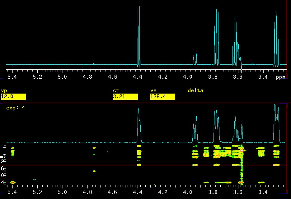 |
|
top: CSSF 1D-TOCSY with
selective excitation of
βH1
at 4.4 ppm and a mixing time of 0.120 seconds |
An expansion is shown here, simply to emphasize the difference in quality of the 1D vs. the 2D version. Around 3.6 ppm there is actually a triplet (βH4) and a d x d x d (8 lines βH5) very close together.
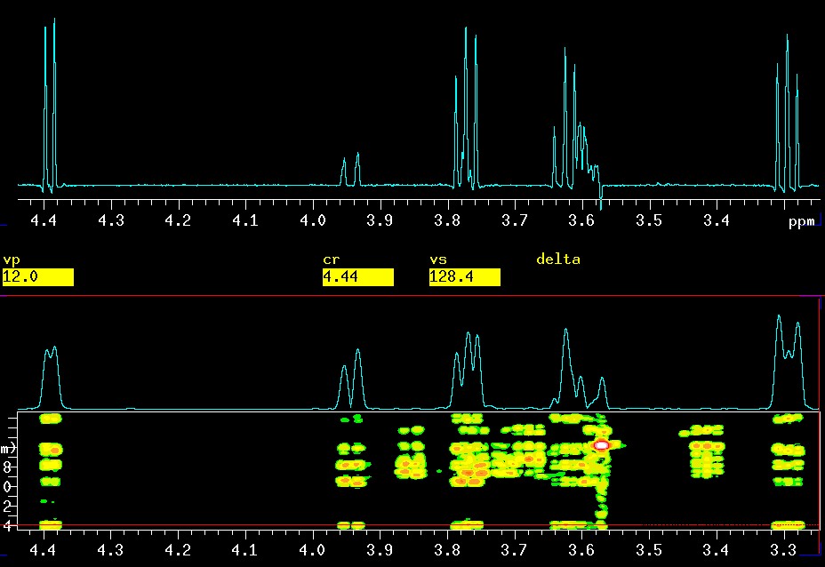 |
|
top: CSSF 1D-TOCSY with
selective excitation of
βH1
at 4.4 ppm and a mixing time of 0.120 seconds |
The selection of appropriate values for the mixing time (mix) has been discussed earlier and the effect of mix on peak build-up with 2D-GTOCSY data can be seen here. The picture below shows the effect of mixing time in the CSSF 1D-TOCSY when the αH1 signal at 5.4 ppm is selectively excited. At 0.010 seconds there is virtually no peak visible but at 0.030 the αH2 at 3.58 appears and at 0.050 αH3 at 3.68 ppm. αH4 at 3.42 ppm is not far behind αH3 in building up intensity but it is slower. At about 0.110 seconds αH5 at 3.71 and the two αH1a/b at 3.86 and 3.76 ppm appear. The reason that 5 and 6 appear almost identical in buildup has something to do with the fact that αH5 is a very low intensity signal due to its d x d x d splitting.
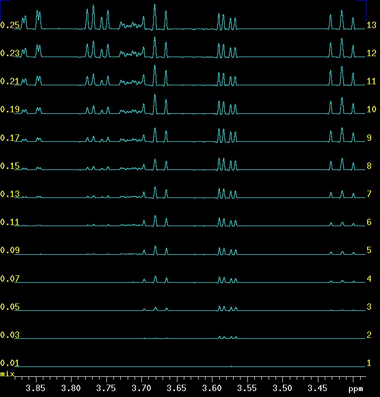 |
|
effect of mixing time (mix) on peak build-up when αH1 is selectively excited |
Another way to look at these data is in a horizontal display. This way it is quite obvious that there are delays in the protons further away from the αH1 which was a selectively exited. This information has the capability to help with assignments!
 |
|
effect of mixing time
(mix) on peak build-up when
αH1
is selectively excited; from top to bottom:
|
How to use the CSSF techniques
In these notes, the TOCSY technique is used. The 1D- NOESY works very similar (exceptions are noted here).
The EZ-NMR panel contains a button for each technique so it can be started easily:
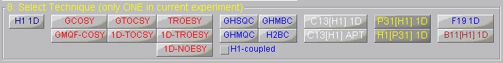
Clicking on the 1D-TOCSY button loads all relevant parameters for the experiment with the exception of two that need to be entered in the window shown below. In general, it is best when the extra windows are dragged over to the second monitor.
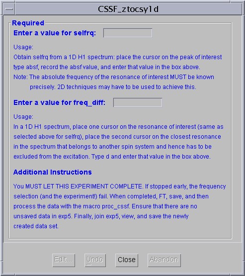 |
What
has to be entered is described in detail in the window so this does not have to
be repeated here. If the chemical shift difference between desired and undesired signals is small, the precise chemical shift has to be known. In this case it may well be necessary to run one or more 2D techniques first to establish this before the 1D can be run successfully. The spinner is turned off automatically for good reasons: spinning degrades the spectral quality. NOTE that this experiment must run to completion to be successful. |
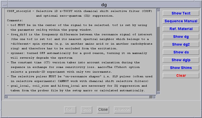
A manual page appears in the second window shown below. It is a fairly comprehensive description of the entire technique but in most cases there is no need to change anything other than the two parameters selfrq and freq_diff.
CSSF 1D-NOESY
Pretty much everything is the same as in the 1D-TOCSY. The main difference is
the longer mixing time (default is 0.400 seconds) and a need to be more careful
and selective with the excitation and exclusion of unwanted peaks. This is
described in quite some detail in the manual page that automatically pops up
when the technique is selected from the buttons. The mixing time cannot be
shorter than 0.135 seconds.
Acknowledgments
The CSSF 1D techniques were brought to our attention by Mickey Richards (Lowary
group). Mickey was also very helpful in testing and suggesting improvements.
Dr. Sara Duncan (Astra Zeneca)
kindly provided the pulse sequences.
A lot of work to adapt to our systems was
carried out by Mark Miskolzie.
Literature
CSSF P.T.
Robinson, T. Nghia Pham, and D. Uhrin, J. Magn. Reson. 170, 97-103
(2004).
ZQ suppression M.J. Trippleton and J.
Keeler, Angew. Chem. Int. Ed. 42, 3938-3941 (2003).