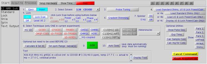
5. EZ NMR S+A
The EZ NMR S+A (Setup and Acquisition) panel is an entirely in-house created panel. This panel provides a simple central interface for acquisition of routine experiments. The panel should be used as a To Do List by following the numbered steps (simply count to ten!).
Notes:
- In a multi-user environment it is unknown what the last user left behind (z0, shims, probe tuning, solvent, etc.) and may not be suitable for your sample
- The correct solvent is fundamental to the proper setup of the instrument
- 20 solvents are available in the drop-down list
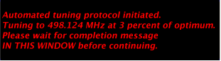
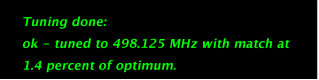
- Allow the spectrometer time to complete probe tuning, loading standard shims, finding the lock, and gradient shimming before proceeding to the next step. Completion messages are provided and failure to wait will hang the system.
|
Figure 5.15 : EZ NMR S+A panel |
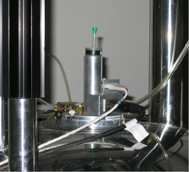
5.1 Step 1 - Inserting a sample
 |
|
Figure 5.16 : Inserting the sample |
|
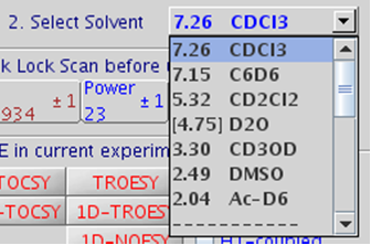
5.2 Step 2 – Select Solvent
 |
|
Figure 5.17 : Solvent drop-down menu |
|
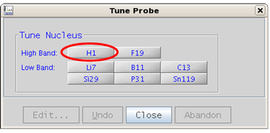
5.3 Step 3 – Probe Tuning
|
All parameter sets are based on a properly tuned probe. Failure to tune can result in partial or complete loss of NMR signals in your experiment.
Experiments that involve a hetero or X nucleus (where X can be C13, P31, B11, etc.) both the X nucleus and H1 need to be tuned and in that order!
Examples of experiments that need both the X nucleus and H1 tuned: APT, C13[H1] 1D, gHSQC, gHMBC, B11[H1] 1D, H1[P31] 1D, etc. but not F19.
| Tuning depends on: | |
|
|
Figure 5.18 : Tuning with ProTune. Top - Probe Tuning button, bottom - Tune Probe pop up window |
Tune Probe
|
5.4 Step 4 – Load Standard Shims, z0, Lock Power|Gain
Why lock? Every magnet slowly drifts (field drift) to lower magnetic field strength, typically 1 to 5 Hz/hour. To achieve frequency stability over the duration of an experiment (16 hours or more for some 2D, days for 3D, 4D, 5D!), FT spectrometers use the deuterium signal of the solvent as an internal lock. Drift compensation and stability is achieved through comparison of the spectrometer frequency with the lock signal frequency.
The amount of deuterium is quite different in CDCl3, D2O, and CD3OD. Therefore, lock power and lock gain are solvent/spectrometer-dependent (use EZ NMR S+A button 4c: Display z0…. or enter z0 on the vnmr command line to run the z0 macro).
Some solvents like CD3OD have two deuterium signals. Locking on OD is difficult, therefore locking on CD3 is recommended, “much more likely to happen” and assumed throughout these notes. If locked on OD, the spectral window and referencing will be off by ca. 1.5 ppm and gradient shimming may fail.
Loading Standard Shims and Automated Locking step-by-step
| Figure 5.19: Load Standard Shims, z0, Lock Power | Gain | |
|
|
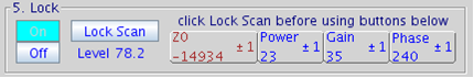 |
Figure 5.20 : Lock Control |
5.4.1 Locking manually step-by step
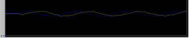
|
Figure 5.21 : Lock Scan (far off resonance) |
- change the lock frequency by clicking on the z0 button until a lock signal is observed as a wavy line
- the middle mouse button toggles 3 sensitivity settings of the z0 button
- if necessary increase Lock Gain first, and then if necessary increase Lock Power
|
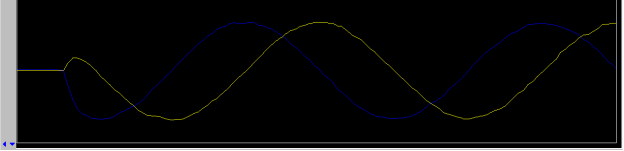
Figure 5.22 : Lock Scan (off resonance) |
- change z0 to reduce the number of “frequency beats” as shown below
|
|
Figure 5.23 : Lock Scan (approaching on-resonance) |
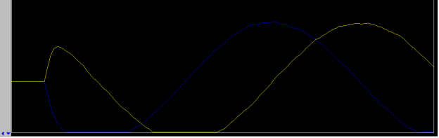
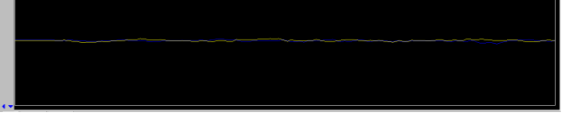
- change z0 until on resonance: the lock signal will be similar to that shown in the figure below, a “plateau”
|
Figure 5.24 : Lock Scan (on resonance) |
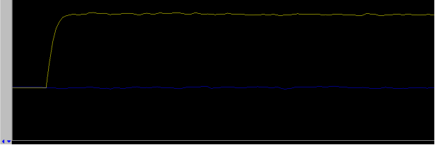
- click on the button Lock On in 5. Lock panel. Further adjustments to z0 are no longer necessary
- adjust lock phase if necessary to maximize Lock Level then turn off Lock Scan
- for systems such as the u500, i600, or v700 (VNMRS console) adjust lock phase with the yellow lock line on top, all other instruments (Inova and Mercury+) only have a single yellow lock line
|
Figure 5.25 : Lock Control (on resonance, locked) |
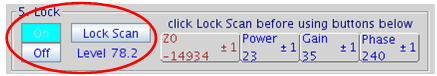
If not successful turn Lock Off and/or continue to search for the z0 frequency. Once locked, avoid high lock power which causes saturation, i.e. more power flows into the sample than can be dissipated through relaxation processes resulting in sample heating, poor quality spectra, and potentially no lock.
Use information from z0 macro to estimate suitable values.
General guidelines:
- If needed, increase lock gain and when necessary increase lock power.
- The Lock Level should be between 80 and 100 (but not over 100) for a shimmed sample otherwise the lock may be lost under the effect of gradients.
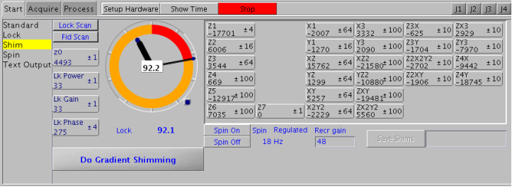
5.5 Step 6 – Gradient Shimming
Purpose of Shimming: optimize the homogeneity of the magnetic field by using shim gradients: Z1(linear), Z2 (squared), X, Y and many more
(There are as many as 28 shims available on some instruments!).
|
|
Figure 5.26 : Gradient shim button and gradient shimming message. |
|
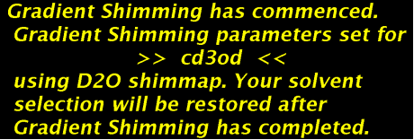
Gradient shimming is an automated shimming protocol that will adjust shim gradients Z1 to Z4 in a very short period of time and is the recommended method of shimming a magnet.
Only if gradient shimming fails (i.e. gradient shimming fails to converge, all peaks within the spectrum are split, etc.), use manual shimming:
- change Z1 to obtain maximum lock level on “speedometer”
- change Z2 to achieve the same, then return to Z1
- repeat until no further improvement can be achieved
- the middle mouse button changes the sensitivity of the shim and lock buttons (i.e. values of 1,10, or 100 are selectable)
- if shim changes are large, re-optimize lock phase
|
Figure 5.27 : Start Tab - Shim panel |
5.6 Step 7 – Spinner
Turn spinner on if desired.
|
Figure 5.28 : Spinner button |

Notes:
- On most modern NMR spectrometers the improvement seen in magnetic field homogeneity from spinning a sample is very minor.
- The system will turn the spinner off for some techniques, i.e. all 2D experiments and selected 1D experiments.
5.7 Step 8 – Select Technique
Common 1D and 2D experiments can be selected as shown in the following Figure:
|
Figure 5.29: EZ NMR Techniques |
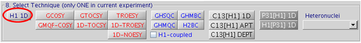
Note: It is recommended to always record a H1 1D before recording any 2D or heteronuclear experiments. The time requirement for a H1 1D is minimal and this allows one to check
- if the sample is really worthwhile (purity, concentration, etc.)
- if the homogeneity of magnetic field (shimming) is what it should be
- if other adjustments are necessary (spectral width, nt, etc.)
Heteronuclear techniques (Li7[H1] 1D, B11[H1] 1D, F19 1D, Si29[H1] 1D, Si29 gHSQC, Si29 1D, Sn119[H1] 1D, etc.) can be selected from the Heteronuclei drop down menu.
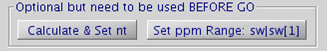
Optionally one can make adjustments to the selected technique prior to starting the experiment. For example a H1 1D:
|
Figure 5.30 : Optional adjustments for selected technique |
Calculate & Set nt Calls macro to calculate number of transients (nt) based on sample concentration which is calculated from user input. For example, calculating nt for a sample with a solute concentration of 70 mM. The system will prompt: What is the molecular weight? 370 How many mg of the compound? 18 The default of 16 scans or nt=16 is set. |
Set ppm Range: sw|sw1 Calls a macro to calculate the spectral width (sw and/or sw1) based on user input. For example setting the sweep width for H1 1D from 8.4 ppm to 1.2 ppm. The system will prompt: Enter desired low field (highest ppm) limit: 8.4 Enter desired high field (lowest ppm) limit: 1.2 |
5.8 Step 9 – GO!
|
Figure 5.31 : Start the NMR experiment! |

Press the very large GO! button to start the experiment. Sit back, relax, your experiment is in progress.
As data becomes available the user can start processing the data. See section 6 for details.
5.9 Step 10 – Auto Save
|
Figure 5.32 : Auto Save |
Included in the EZ NMR S+A to do list, but optional, is Auto Save.
Auto Save will:
- save the data for the user in their absence
- save the data in the current working directory using a standard naming format (see section 7.2 for details on the standard naming format)
- save the data as long as the experiment is running
- save the data as long as the instrument does not encounter an error
- save the data when the experiment finishes